
A FOREST BUSINESS SCHOOL BRIEFING
Woods to Wheels: Every Gallon Counts
Fuel use in timber harvesting and log trucking across the United States and Canada
Arkansas equipment demonstration, 2011 · Steve Bick
About this briefing
Prepared for state forestry agency staff and private-sector stakeholders briefing policymakers on the effects of rising fuel costs. This web edition brings together the revised paper’s evidence, six complete tables, figures and interactive fuel calculations.
Cited studies are linked throughout for readers who want to consult the original research. Unpublished sources are identified in the reference notes.
Executive summary
This briefing assists state forestry agency staff and private sector stakeholders who have been asked to brief policymakers on rising fuel costs and their effects on the forestry sector. It brings together evidence on in-woods timber harvesting and log trucking, compares operating conditions across U.S. regions and Canada, and identifies the information needed to evaluate potential cost relief. Fuel use depends on the work performed, the volume produced and the distance wood travels. These distinctions are essential when translating contractor experience into policy estimates.
The regional evidence spans southern ground-based crews, Northeast contractor records, Lake States business surveys, western harvesting and haul systems, and Canadian inventories. Kenney’s two-year sample of six crews in southern Alabama and northeastern Florida averaged 0.51 U.S. gal/ton for in-woods work, excluding outbound haul. Southern contractor records put on-road use near 0.8 gal/ton. Vermont field trials reported 1.6 and 2.4 gal/cord, and the unpublished northern New York study reported 0.61–1.78 gal per green short ton for roundwood through loading. A Minnesota survey reported a screened median of 1.20 and mean of 2.93 gal/cord equivalent for off-road business fuel. Western cases distinguish ground, skyline and helicopter systems; Canadian inventories retain cubic-meter denominators and explicit green-density assumptions for weight conversions. Comparisons require matched systems, units and activity boundaries. The national scenarios use illustrative regional coefficients. [S05, S06, S10, S12, S15, S16, S17, S18, S45, S46, S47, S48, S49]
The modeled 2022 benchmark covers sawlogs, veneer logs, pulpwood and composite products. Its central case is 170 million gallons and $659 million for harvesting and 229 million gallons and $1.13 billion for log trucking. The combined central case is 399 million gallons and $1.79 billion in nominal 2022 dollars. The joint low and high cases span about 191–812 million gallons and $0.74–$4.13 billion. These are conditional scenarios for the selected products. Alaska’s production is documented separately and its fuel is omitted from the totals. Hawaii is included geographically in the source’s Pacific Southwest grouping and has no standalone fuel estimate. The trucking calculation assumes a truck-equivalent first haul where dispatch and modal share data are missing. The broad range primarily reflects trucking assumptions, measurement boundaries and mass conversion. [S05, S06, S08, S15, S16, S17, S18, S19, S20, S22, S23, S24]
Two anonymous Northeast archival cases yield 1.51 (New York) and 0.98 (Maine) U.S. gallons of off-road fuel per green short ton. They describe mixed-product operations from one contractor in each state. Three related publications draw on the same research family; this briefing retains each study’s methods and boundaries and reports the archive cases separately. [S53, S54, S55, S56]
Canadian evidence broadens the operating comparison. Historical eastern and western softwood inventories differ in diesel use per cubic meter. A New Brunswick hardwood-company case converts to about 1.00 U.S. gallon per green short ton using the study’s green-log density as a proxy. Each comparison retains its conversion assumptions and original units. The national fuel scenarios use U.S. harvest volumes exclusively. [S46, S47, S48, S49]
The available public data do not support a defensible estimate of annual fuel expenditures for timber harvested on farms versus elsewhere. The Census of Agriculture measures farm woodland acreage and certain receipts and expenses. Forest Service data measure harvest volumes, geography and broad ownership. Contractor records measure fuel or output for selected operations. The sources lack the common tract identifiers, program-defined farm status and matched contractor records needed to make the split. A farm-woodland acreage share would be a particularly weak substitute, because harvest rates and harvest methods can differ materially across acres and owners. [S21, S25, S26, S27, S28]
USDA’s current Harvest Fuel Relief request for non-Title I commodities seeks aggregate on-farm production fuel evidence. FSA’s published guidance excludes processing and transportation out of the field or to market. The public guidance at review left eligibility and timing for non-Title I commodities forthcoming. A timber-specific interpretation of where production ends, who qualifies and how contracted harvesting would be treated remains unresolved. The broader industry scenarios provide cost context and have no role as estimates of HFR-eligible spending or payments. [S01, S02, S03, S04]
1. Scope and research approach
The policy question
On October 19, 2026, USDA announced a one-time Harvest Fuel Relief program of up to $8 billion, through the Farm Service Agency and the Commodity Credit Corporation. The announcement described proportional assistance for a portion of modeled losses in the 2026 crop year. The FSA page differentiates Title I and non-Title I commodities. It states an October 16 acreage-on-file date for Title I acreage, and treats non-Title I commodities separately. For the latter, the agency prefers aggregate industry evidence on production fuel. The New Jersey Department of Agriculture publicized the request for consumption and pricing data, and Wisconsin public radio documented industry advocacy for timber and logger inclusion. The available official materials do not settle timber eligibility. [S01, S02, S03, S04]
Policymakers need information about fuel consumption and potential cost relief. This briefing separates harvesting from trucking, compares regional evidence and examines the data required to distinguish timber harvested on farms from timber harvested elsewhere. Public FSA materials establish the program context; complete timber-specific instructions remain necessary to clarify administrative definitions. [S01, S35]
For a program decision, the fuel boundary and the party eligible to claim it both matter. Felling and moving wood to a landing serve different functions from transporting it over the road to a mill. Landing processing, truck loading, movement by internal roads and in-woods chipping warrant explicit treatment if USDA issues timber-specific guidance. A landowner may receive stumpage, a logging contractor may buy fuel, and an independent carrier may haul the load. Those parties may appear on the same transaction without incurring the same expenses. Contract language can also shift the cost of a price increase while leaving the fuel invoice in the carrier’s name. NAICS 113310 classifies establishments by activities such as cutting timber, cutting and transporting timber, or producing chips in the field. The code describes the establishment’s business activity. A tract’s farm status and the claimant’s eligibility require separate evidence. [S44]
The review combined Forest Service and FIA inventory, TPO and harvest-utilization sources, USDA and state program documents, NASS, EIA, university repositories, journals, extension materials, association reports and forest industry surveys. English- and French-language searches covered U.S. and Canadian regions, in-woods fuel, harvest productivity, contracting, log hauling, truck utilization and farm woodland. Relevant Canadian sources included Athena inventories, FERIC/FPInnovations references, conference proceedings and federal life-cycle methods. Key studies were traced to original publications and compared with subsequent syntheses, including the 2025 transportation-industry comparison. Steve Bick supplied data from past studies, including the unpublished 2015 study commissioned by NYSERDA and the ESF-DOE contractor archive. The archive audit checked spreadsheet formulas and selected source forms, distinguished reported totals from estimated process allocations, and retained traceable cases for anonymous aggregate reporting. The calculation workbook records geography, vintage, sample, methods, units and stage. The source register identifies abstract-only and summary-only records and their limits. Coverage reflects the materials retrieved through November 17, 2026; original FERIC coastal and western reports remain retrieval priorities. The archive checks establish arithmetic and provenance within the available records; business-account certification and independently metered fuel measurement were outside the review’s scope. [S05, S06, S07, S08, S09, S10, S11, S12, S13, S14, S15, S16, S17, S18, S19, S20, S21, S22, S23, S24, S31, S32, S33, S34, S35, S36, S37, S38, S39, S45, S46, S47, S48, S49, S50, S51, S52, S53, S54, S55, S56]
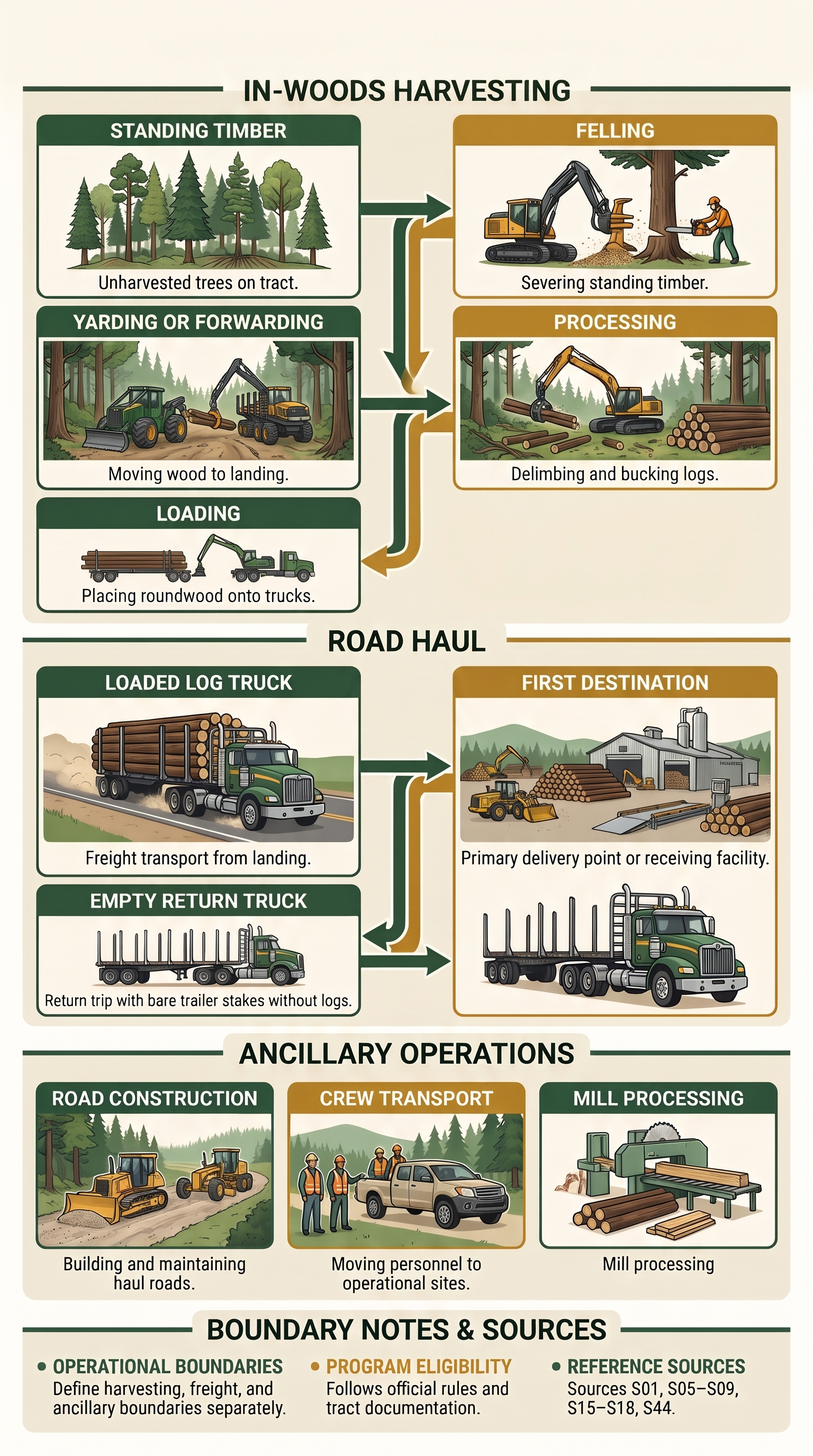
The modeled woods stage covers felling, yarding or forwarding to the landing, processing and loading based on the best comparable evidence. Some studies include limited incidental bulldozer or in-woods vehicle fuel. The model makes no separate allowance for road building or upkeep, lowboy moves, support vehicles or grinding. The road stage covers modeled landing-to-first-destination log freight and associated empty travel. It excludes secondary mill-to-mill movement, procurement pickups and rail or water fuel. A business that subcontracts haul may pay a rate that embeds fuel. Counting both that embedded charge and the carrier’s fuel purchase as fuel spending would double count. [S05, S06, S07, S08, S09, S15, S16, S17, S18] Figure 1 illustrates the separation between the woods stage, first haul and ancillary work.
Diesel dominates the documented in-woods harvesting equipment and haul cases. Other fuels can matter on particular jobs. Northern California redwood work documented gasoline chainsaws and aviation fuel for helicopter yarding, alongside diesel used in ground equipment and trucks. A high-fuel helicopter observation is a mixed-fuel example and is excluded from diesel scenario calibration. Available sources offer too little paired usage and price information to construct national estimates for gasoline, aviation fuel, biodiesel blends or renewable diesel as separate categories. Defining those purchases by activity and product is a prerequisite to adding them. [S15, S23, S24]
2. United States regional evidence
What the observed fuel rates show
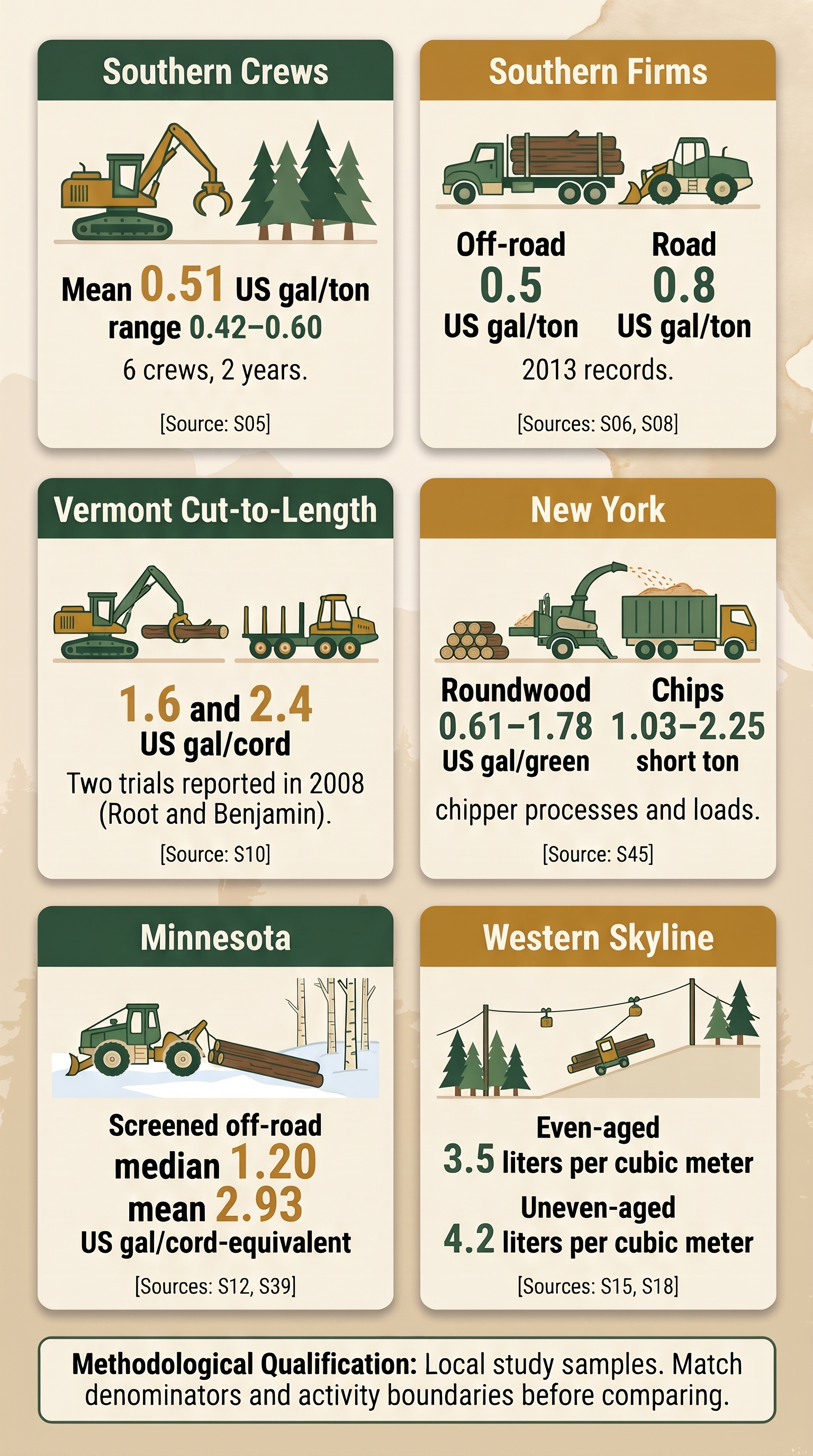
Southern ground-based crews. Kenney’s weekly sample comprised feller-bunchers, skidders and loaders, with a few ancillary machines including bulldozers, in-woods trucks, delimbers or processors where reported. The crews worked thinnings and clearcuts in 5- to 18-inch diameter material. Sites were under 35% slope and mostly under 15%. Crew means were 0.42–0.60 gal/ton. A separate tract sample averaged 0.65 gal/ton. It covered nine crews in Alabama, Georgia, Louisiana, North Carolina and Ohio, and its reported range of 0.37–0.94 includes a low observation missing felling fuel. The study’s calendar is reported here as two years before the May 2015 thesis. The results describe the recorded systems and samples in their study period. [S05] The six-crew weekly sample covered about 486,000 tons over two years. The thesis reports production in tons without an explicit 2,000-pound definition in the relevant methods and results; this briefing uses green U.S. short tons as the working interpretation. [S05]
Southern trucking. Baker interviewed 23 logging firms across six states and obtained detailed 2013 production and cost records from 17. Firms reported about 49 one-way miles, 5.1 mpg, 0.5 gal/ton off road and 0.8 gal/ton on road. They contracted roughly one-third of hauling. The sample was small and included comparatively large operators. Conrad later analyzed 909 deliveries using route information and simulated additional operating variables. His mean haul was 49.5 miles one way, modeled mean payload 28 green short tons, modeled loaded share 44.3%, and assumed fuel economy 5 mpg. Those inputs imply 0.80 gal/ton. The agreement is a check on the magnitude for these study settings. It gives no statewide coverage of all contractors or routes. [S06, S08, S09]
Northeast and Lake States. Root and Benjamin’s Vermont field trials, reported in the 2008 ECANUSA proceedings, combined a dangle-head harvester and a forwarder. The lower rate was for mostly spruce and white pine sawlogs. The higher rate was for a hardwood job, so species and job effects cannot be isolated. Published hardwood scenarios for the Northeast also find that partial cuts and clearcuts produce different relative efficiencies for chainsaw-based and machine-based harvesting systems. A Minnesota survey’s mean-to-median difference shows how strongly a small sample of business ratios can depend on the distribution of company size and production. Minnesota’s reported on-road average of 33,248 gal per responding business includes a different set of respondents from the off-road figures and may include other travel. The Northeast association’s published 2.1 gal/ton member estimate deserves follow-up. Its denominator and whether it captures trucking, support equipment, or other operations are insufficiently documented for use in the model. [S10, S11, S12, S13, S14, S39]
Northern New York roundwood. Steven Bick’s unpublished 2015 study, commissioned by NYSERDA, drew on records from northern New York logging contractors. NYSERDA chose to keep the study unpublished. Twelve contractors supplied data and eight provided records complete enough for the analysis overall. Cutting, skidding, processing and loading roundwood took 0.61–1.78 gallons per green short ton (0.56–1.64 green short tons per gallon). The figures end at truck loading, and green tons are treated as U.S. short tons. Fuel included diesel and diesel–kerosene blends. Chipping also occurred on these harvests: it adds processing work and fuel while the chipper simultaneously loads chips into the truck. The reported roundwood range and the separate chip-production rates below retain those distinct activity boundaries. The study reports a roundwood range only. [S45]
That range includes the Northeast central scenario of 0.82 gal/ton. Its upper end is 42% above the model’s 1.25 gal/ton high case. The contractor records show that individual operations can exceed the modeled regional rate. The Northeast scenario retains its existing inputs because the study provides neither a roundwood mean nor a production-weighted regional estimate. The same study reports 1.03–2.25 gal/ton for fuel chips, averaging 1.51 gal/ton (0.66 green short ton per gallon). That figure includes chipping directly into a truck at the landing and is used here only for the chip-production comparison. [S45]
Western operational differences. CORRIM’s Pacific Northwest examples provide staged process inventories and a 57-mile haul input for some cases. Mason and colleagues’ Washington study used a six-axle long-logger sample payload of 58,835 lb and reported fuel economy near 5.1 mpg. In northern California redwood operations, Han and colleagues found that extraction consumed much of stump-to-truck fuel. A skyline example used 3.5 L/m³ for an even-aged entry and 4.2 L/m³ for an uneven-aged entry. The paper also reported average hauls of 52 km for sawlogs and 76 km for biomass. Those results point to differences between forest types, assortments and markets within western states. The recent Inland Northwest lumber inventory uses a mill functional unit, including sawmill rolling stock, so those mill diesel entries cannot serve as woods fuel rates. [S15, S16, S17, S18, S32] Figure 2 summarizes these observed rates while retaining each study’s units and operating boundary.
Geographic coverage and interpretation
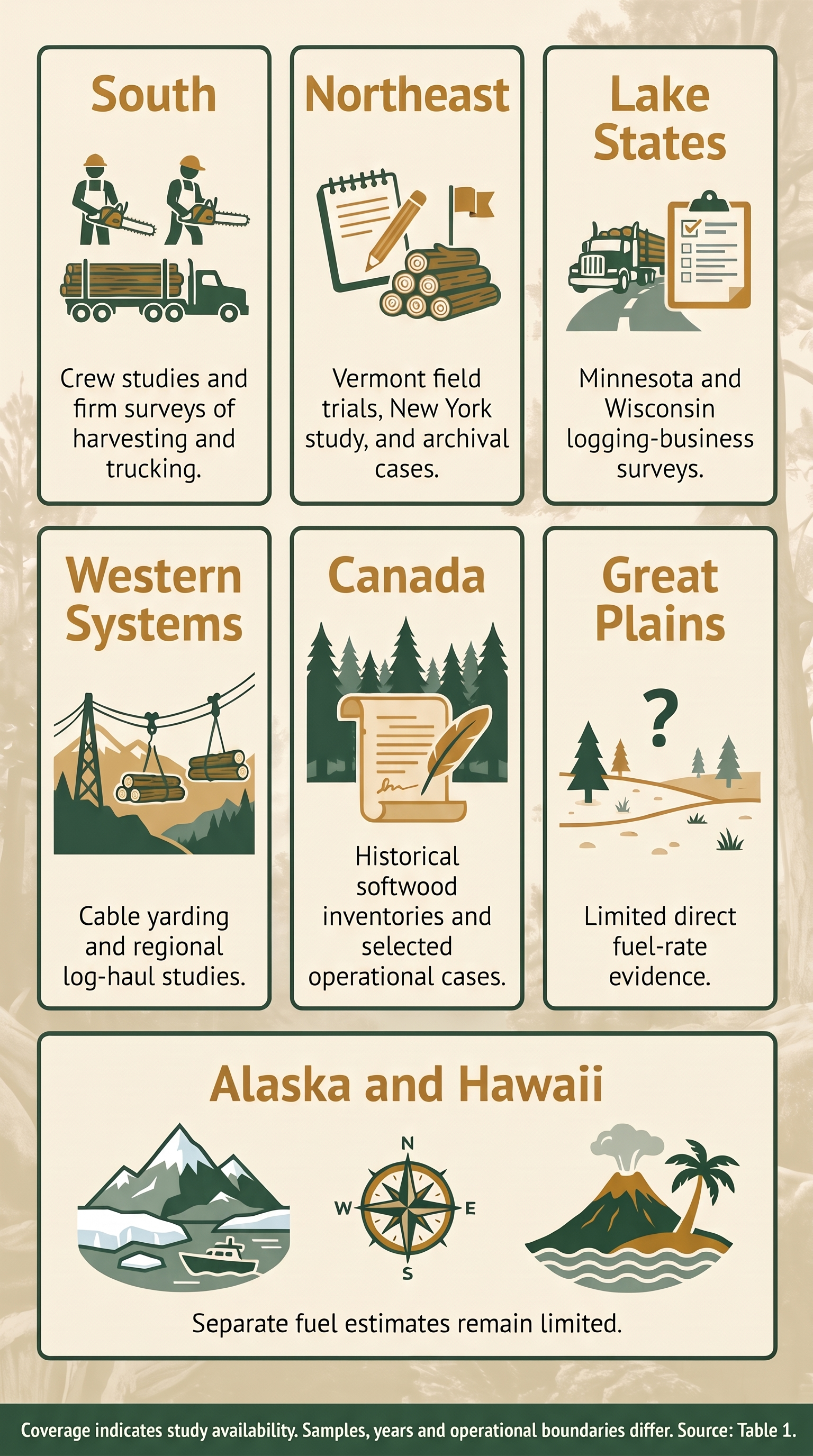
The numerical geography follows the U.S. Forest Service 2022 appendix. It uses nine subregions and a separate inventory assigns all 50 states. In this system, the Lake States are Michigan, Minnesota and Wisconsin within North Central. The Southeast includes Florida, Georgia, North Carolina, South Carolina and Virginia. The South Central covers Alabama, Arkansas, Kentucky, Louisiana, Mississippi, Oklahoma, Tennessee and Texas. The Intermountain group includes Arizona, Colorado, Idaho, Montana, Nevada, New Mexico, Utah and Wyoming. The Great Plains group includes Kansas, Nebraska, North Dakota and South Dakota. Pacific Northwest means Oregon and Washington, including their inland areas. Pacific Southwest groups California and Hawaii. Alaska has its own entry. The Northeast includes the Mid-Atlantic states assigned by the source, including West Virginia, and North Central also contains the remaining five states listed in the workbook. These are accounting geographies. Conditions and freight markets cross state lines. [S19, S20, S21, S33, S34] Table 1 summarizes regional evidence and its interpretation; Figure 3 provides a visual guide to its uneven coverage.
| Area | Evidence and implications |
|---|---|
| Northeast | Vermont field data, northern New York contractor records, eastern hardwood models and Northeast industry evidence. [S10, S11, S14, S45] Small or selective tracts, tree size and extraction distances can change output per machine-hour. Mill closures or product-market changes can shift loaded haul and route length even when the harvest system is unchanged. |
| Lake States and other North Central | Minnesota and Wisconsin contractor surveys, modeled eastern hardwood evidence and Ohio tract records. Forwarding, winter access and road restrictions can change productivity and the mix of projects across seasons. Separate Michigan fleet data and comparable fuel records elsewhere are needed for state rates. |
| Southeast and South Central | The strongest measured-volume and fuel records in the review, particularly for mechanized ground-based crews. Pine plantations, thinnings, mixed hardwoods and wet sites require different operations. A mill closure can raise trucking fuel independently of woods fuel. |
| Pacific Northwest | Historical Pacific Northwest process inventories and a direct Washington fleet survey support sensitivity to cable versus ground systems, truck configuration and payload. Grade, road surface and empty travel also matter. A west-side Douglas-fir case does not represent inland Oregon or Washington. |
| Intermountain | Idaho and Montana have wood production and industry series. Corridor and mill catchments extend outside state lines. Restoration and small-diameter wood can have low output per hour and limited destinations. Fuel coefficients are transferred and uncertain in the Rockies and Southwest. |
| Great Plains | The Black Hills evidence straddles South Dakota and Wyoming, while most Great Plains states have no direct observations in this review. Public-forest production or mill-capacity figures establish activity. Neither establishes fuel intensity for the whole region. |
| Pacific Southwest | Northern California redwood studies establish differences among ground, cable and helicopter systems. A California trucking and price proxy serves the aggregate. Hawaii’s forestry division documents local timber and markets. Comparable commercial volume and first-haul fuel are unavailable separately in the sources examined. [S42] |
| Alaska | Harvest-utilization observations and production series document logging activity. Road-only, short road plus water, and other supply configurations require separate records. The Forest Service reports 26.4 million cubic feet of all-product roundwood in the 2022 Alaska reporting period. The workbook retains that volume and leaves both fuel estimates blank. [S20] |
The regional price effect is distinct from the operational effect. In 2022, average on-highway diesel was $4.683/gal in the Gulf Coast district and $6.028/gal in California. A firm buying bulk fuel or using a fleet contract may have paid a different amount. The model assigns selected EIA price districts to forestry subregions, including New England for the Northeast and Gulf Coast for South Central, as representative prices. These assignments do not replicate the distribution of deliveries or purchases within the regions. [S23, S24]
Northeast contractor records and the published research family
The Bick-supplied ESF-DOE archive and three related journal papers address complementary Northeast research questions. The archive permits selected physical fuel-to-output calculations. The papers apply life-cycle or economic models to related forest-biomass systems. This briefing keeps these records and publications separate and retains the unpublished 2015 New York study as a distinct comparison. Possible record overlap requires further checking before any pooled analysis. [S45, S53, S54, S55, S56]
Published findings and their boundaries
Quinn and colleagues (2020) studied forest-biomass feedstocks using records from nine contractors in New York, Maine, Massachusetts and Vermont over 2013–2019, covering 79 harvest periods. Harvest periods may include repeat observations of a tract. Most systems were whole-tree operations; one used a hybrid cut-to-length approach. The functional unit was a green metric tonne (Mg), with 50% moisture assumed in the model, through roadside loading rather than delivery to the user. Lifecycle inventories include equipment, other inputs and support activities as well as fuel. The resulting greenhouse-gas quantities are allocation-dependent impacts across several inputs. Recovering physical fuel use requires the underlying fuel inventory and activity boundaries. [S53]
The public supplement explains that estimated landing-machine fuel is deducted from total stump-to-truck fuel to derive a residual for felling, skidding and best-management-practice work. Those components are estimated allocations. Its contractor process table and model-input table show an apparent scaling discrepancy, while clean-chip aggregate values differ between two main-text tables. The cause was not established in this review. The briefing therefore retains the reported components separately, including their differing product denominators. Resolving the discrepancies requires source-data reconciliation before unit conversion. [S53]
Ha and colleagues (2022) evaluate modeled economics of clean- and dirty-chip supply chains using related historical whole-tree records, including hauling economics. Ha and colleagues (2024) extend the research family with a stochastic, long-horizon techno-economic analysis. The 2022 study reports green-mass economics and the 2024 study reports dry-mass economics, so cost comparisons require an explicit moisture conversion. Publisher abstracts and bibliographic records were verified for both papers, but their full methods were not available for this review. Their contribution here is the published economic framing and bibliographic context. [S54, S55]
Selected archival fuel and production calculations
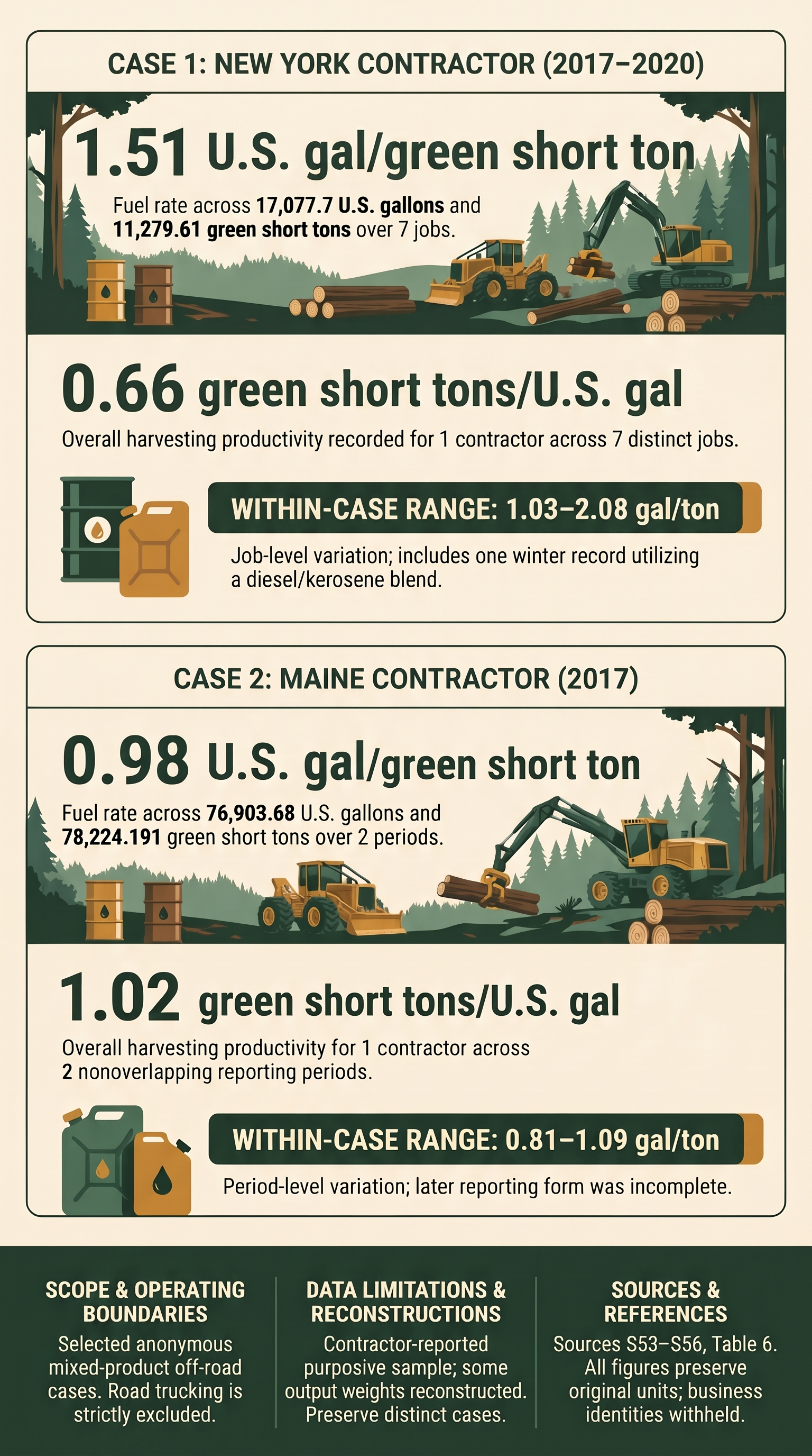
Table 2 reports two anonymous contractor cases selected because their total-fuel and total-product arithmetic could be traced and checked. Ratios divide each case’s summed reported off-road gallons by its summed green short tons, weighting records by production. The source forms and pounds-to-tons calculations support U.S. liquid gallons and 2,000-pound short tons. Some product weights were directly recorded; others were reconstructed from board feet, cords or loads using source-specific factors. Each record retains its source-specific moisture or density assumptions. [S56] Figure 4 displays the two case summaries alongside their boundaries and limitations; its rates are calculated from contractor-reported records.
| Anonymous case and coverage | US gal per green short ton | Green short tons per US gal | Record range US gal/short ton |
|---|---|---|---|
| New York case Seven jobs, 2017–2020 One contractor | 1.51 | 0.66 | 1.03–2.08 |
| Maine case Two nonoverlapping periods, 2017 One contractor | 0.98 | 1.02 | 0.81–1.09 |
Source: Bick-supplied ESF-DOE contractor archive, selected records, unpublished reanalysis for this briefing [S56]. Rates are rounded; record ranges describe variation within each case, not regional uncertainty bounds. Road trucking is excluded. Product mix and support-work boundaries differ from roundwood-only comparisons, and neither case is a probability sample.
New York case. Seven distinct jobs from 2017–2020 total approximately 17,078 reported off-road gallons and 11,280 green short tons. The exact aggregate inputs, retained in the calculation workbook, produce 1.5140 gal/short ton and its reciprocal, 0.6605 short ton/gal. One winter record explicitly uses a 50:50 diesel–kerosene blend, so the aggregate is described as off-road fuel. Two jobs whose fuel was explicitly contractor-estimated were excluded. Pre-2015 records were also excluded because possible overlap with the earlier unpublished study has not been resolved. The selected denominator includes chips and logs, with some estimated log-mass conversions; the resulting rate covers that mixed output. [S56]
Maine case. Two nonoverlapping reporting periods in 2017 total approximately 76,904 reported off-road gallons and 78,224 reconstructed green short tons. Their aggregate produces 0.9831 gal/short ton and 1.0172 short tons/gal. Products include chips, logs, pulpwood and firewood. Logs and firewood use source conversion factors rather than a matched weight for every load. Minor transcription and mixed-load allocation differences remain, but the checked alternatives do not change the reported two-decimal aggregate of 0.98. The first-period source form was checked; a complete source form for the later period was not located. Both periods describe one business. [S56]
Excluded archive records contain omitted product tonnage or processing fuel, unrelated load-size cells, mismatched row ranges, unexplained invoice reductions, inconsistent log units, land-clearing boundary mismatches, or explicitly estimated chipper fuel. Their use requires reconciling formulas, source records and activity boundaries. Original records remain unchanged. [S56]
3. Canadian regional comparisons
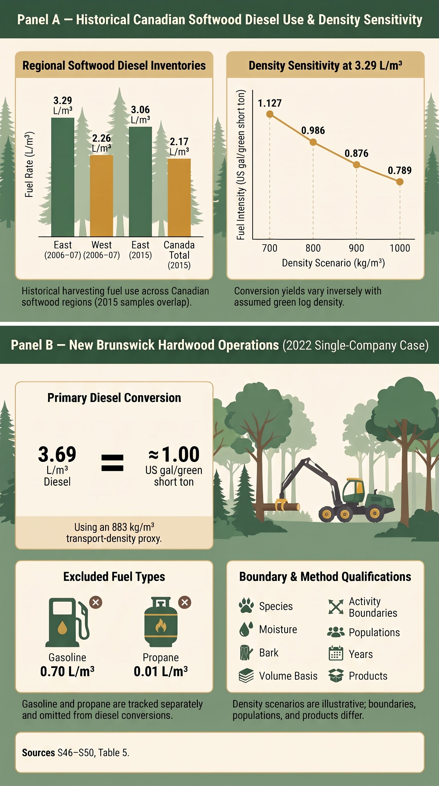
Canadian studies provide additional operating examples with clearly defined years, products and activity boundaries. Table 3 retains original diesel denominators, gives U.S. liquid-gallon equivalents and specifies the density needed for a short-ton comparison. Farm-status fuel measurement remains an evidence gap across these studies. Figure 5 shows how assumed green density changes the conversion and identifies the New Brunswick case’s source-derived density proxy. [S46, S47, S48, S49, S50, S51, S52]
Historical East and West evidence. Athena’s 2009 softwood-lumber inventory used 2006–07 questionnaires from eight eastern forestlands in Ontario and Quebec and four western forestlands in British Columbia and Alberta. Their respective diesel inventories were 3.29 and 2.26 L/m³ harvested. Both cover stump-to-roadside harvesting plus forest management and reestablishment; road construction and outbound road transport are outside this fuel comparison. The results describe those historical samples. [S46]
More recent softwood inventories. Athena’s 2018 reports use 2015 data: five eastern harvesting operators reported 3.06 L diesel/m³ and eleven Canadian operators reported 2.17 L/m³. The national and eastern samples overlap. The national average retains its Canadian coverage, and the 2006–07 and 2015 samples differ, limiting inference about efficiency trends. The harvesting and mill samples have different species mixes, requiring separate density evidence for harvested green mass. [S47, S48]
| Study and observation | Reported diesel L/m³ | U.S. gal/m³ | U.S. gal/green short ton |
|---|---|---|---|
| East, 2006–07 [S46] 8 forestlands | 3.29 | 0.869 | 0.986 at assumed 800 kg/m³ |
| West, 2006–07 [S46] 4 forestlands | 2.26 | 0.597 | 0.677 at assumed 800 kg/m³ |
| East, 2015 [S47] 5 operators | 3.06 | 0.808 | 0.917 at assumed 800 kg/m³ |
| Canada, 2015 [S48] 11 operators | 2.17 | 0.573 | 0.650 at assumed 800 kg/m³ |
| New Brunswick, 2022 [S49] 1 hardwood company | 3.69 | 0.975 | 1.001 at study proxy 883 kg/m³ |
| Quebec hybrid harvesters [S50] 3 machines; harvester only | 1.09–1.34 | 0.288–0.354 | 0.327–0.401 at assumed 800 kg/m³ |
| Quebec non-hybrid comparator [S50] Harvester only | 1.59 | 0.420 | 0.476 at assumed 800 kg/m³ |
Table 3 notes. The common 800 kg/m³ density is an analyst-selected comparison scenario. Its column shows calculated illustrations whose applicability depends on matching species, moisture, bark and volume basis. The New Brunswick 883 kg/m³ value comes from the study’s green-log transport model and serves as an extraction-volume proxy. The displayed rates cover diesel only. The workbook preserves formulas and a 700/800/900/1,000 kg/m³ sensitivity grid. [S46, S47, S48, S49, S50]
New Brunswick hardwood case. Zahabi and colleagues report 2022 production of 305,000 m³, including bark, from one logging company using machine-based harvesting. Its resource-extraction inventory is 3.69 L diesel/m³, plus 0.70 L gasoline and 0.01 L propane. The equipment boundary includes in-woods trucks and self-loaders as well as harvesting machinery. Applying the paper’s 883 kg/m³ green-log transport density to extraction roundwood gives 1.001 U.S. gal diesel/green short ton, approximately 1.00, or 0.999 green short ton/U.S. gal. The separately calculated gasoline rate is 0.190 U.S. gal/green short ton; it is reported separately from diesel. The transport density serves as a proxy for this single-company case. The separate 118-km mill-haul activity uses modeled transport inputs. [S49]
Quebec equipment and trucking examples. A 2025 conference abstract reports 1.09–1.34 L/m³ for three hybrid harvesters, versus 1.59 L/m³ for a non-hybrid comparator. These are machine-only rates with no forwarder fuel and limited methods available in the abstract. Separately, a hybrid-truck study reports diesel operation up to 72 L/100 km and hybrid operation at 63 L/100 km, equivalent to 3.27 and 3.73 U.S. miles/gallon. The corresponding rates are 0.306 and 0.268 U.S. gal/mile. Payload and loaded/empty allocation are needed before converting these route-specific observations to gallons per delivered short ton. Their route and equipment boundaries differ from the U.S. fleet scenario. [S50, S51]
Evidence gaps and transfer limits. Federal Canadian fuel-LCA guidance uses broad regional inventories because provincial harvesting data are unavailable for its modeling purpose. Provincial case studies provide additional, narrower evidence. Comparable current averages remain unverified for many provinces and territories. The original Sambo 1997 coastal British Columbia and 2002 western ground-based FERIC reports remain priority retrievals; their downstream citations were not adopted as newly verified observations. U.S. farm-status linkage, regional scenario calibration and HFR eligibility each require their own matched evidence. [S52]
4. Units and comparisons
Production and unit conversions
Forest Service table A-41 reports about 13.644 billion cubic feet of total roundwood for the 2022 reporting period. Of this, 11.878 billion cubic feet were sawlogs, veneer logs, pulpwood or composite products. The model excludes fuelwood, poles, posts, pilings and miscellaneous categories so it does not assign an industrial trucking pattern to all roundwood. It also keeps logging residue and other removals out of the denominator. The four product categories are available by broad region and species group in A-41. The workbook applies each broad region’s hardwood and softwood product shares to the corresponding subregional all-product volumes in A-40. The model keeps the published values intact and exposes the allocation formulas. The printed continuation caption for A-40 displays 2016. The official appendix spreadsheet identifies the entries as 2022 and they reconcile with the national 2022 roundwood total. [S20, S21]
The model uses 48, 55 and 62 green pounds per solid cubic foot for hardwood and 39, 47 and 55 for softwood, divided by 2,000 pounds per U.S. short ton. These analyst-selected scenarios reflect wood properties and the importance of green moisture and species mix. A stand’s scale, bark, wood moisture, season and assortment can shift the volume-to-weight relationship. Cords measure stacked volume, and board feet may represent a log-rule estimate; conversion to weight requires matched factors. Primary study results therefore retain their reported units. [S05, S10, S12, S34, S40]
All gallon comparisons use U.S. liquid gallons (3.785411784 liters). A U.S. short ton is 2,000 lb or 907.18474 kg; a metric tonne is 1,000 kg. For a reported rate q in L/m³ and a matching green density rho in kg/m³, U.S. gal/green short ton = q × 907.18474 ÷ (3.785411784 × rho). The reciprocal gives green short tons per U.S. gallon. Green density must match the source’s species, moisture, bark and solid-volume basis. Where it is missing, this report supplies explicitly conditional conversions rather than labeling assumptions as observed ton-based rates.
Regional woods coefficients are analyst-selected scenario inputs. The central southern value of 0.51 gal/ton matches Kenney’s local sample and is extrapolated to larger southern regions. The Northeast 0.82, North Central 0.60, Great Plains and Intermountain 0.70, Pacific Northwest 0.65 and Pacific Southwest 1.00 gal/ton entries are fixed assumptions accompanied by related literature citations. Their exact values lack documented derivations from the cited studies. Retaining these inputs preserves continuity in the scenario calculations; regional calibration remains an important evidence need. The national outputs illustrate fuel-cost exposure under the stated assumptions. [S05, S10, S11, S12, S13, S14, S15, S16, S17, S18]
A separate check demonstrates the importance of green weights. The Forest Service published 113.0 million green tons of southern roundwood pulpwood in a 2022 mill census. Converting the South’s A-41 pulpwood cubic feet with the central generic density assumptions yields 86.25 million green tons. Substituting the published tonnage as a diagnostic, at central southern fuel rates and prices, would add about $153 million to combined modeled cost. The publications use different survey and conversion pathways, so the diagnostic remains separate. Agreement on product classification, source volume and regional green-weight factors would improve the estimate materially. The Alabama and Georgia pulpwood cases in the workbook use the published green ton figures directly, and overlap the corresponding state and national scenarios. [S20, S22, S36, S37]
5. Annual fuel costs and scenarios
Equations and input prices
Harvesting gallons = green short tons × harvesting gallons per green short ton.
Trucking gallons per ton = loaded one-way miles ÷ (all-mile mpg × share of miles loaded × green short tons per load).
Trucking gallons = green short tons × trucking gallons per ton.
Stage expenditures = stage gallons × stage-specific dollars per gallon. Combined expenditures = harvesting expenditures + trucking expenditures.
A carried load travels 49.5 loaded miles in the central Southeast case. Dividing by a 44.3% loaded share gives about 112 total allocated miles, including empty travel. At 5.1 mpg and 28 green short tons per load, that is about 0.78 gallon per ton of delivered wood. A dedicated truck returning empty over the same route gives a 50% loaded share before additional empty positioning. Once empty miles enter through that share, doubling trip mileage separately would count them twice. The calculation assumes all-mile fuel economy, so comparable fleet data must capture idle and road conditions consistently. [S06, S08, S09]
For trucking, the model uses annual EIA tax-inclusive retail highway diesel. For woods equipment, it uses EIA modeled industrial distillate prices, divided by the equivalent gallons per million Btu using 5.825 million Btu per barrel and 42 U.S. gallons per barrel. State prices are averaged without weighting within subregions, with California used for the Pacific Southwest. This gives roughly $3.80–$4.05/gal across most modeled areas in the central case. The industrial series includes a broader set of customers and estimated state sales taxes. It is a price proxy for bulk or dyed diesel, with no universal discount or state-tax deduction applied. The U.S. highway price includes the ordinary federal diesel excise tax and varying state taxes. IRS announcements on temporary dyed diesel relief in 2026 concern a separate federal measure and do not change the 2022 price basis. [S23, S24, S29]
Scenario results
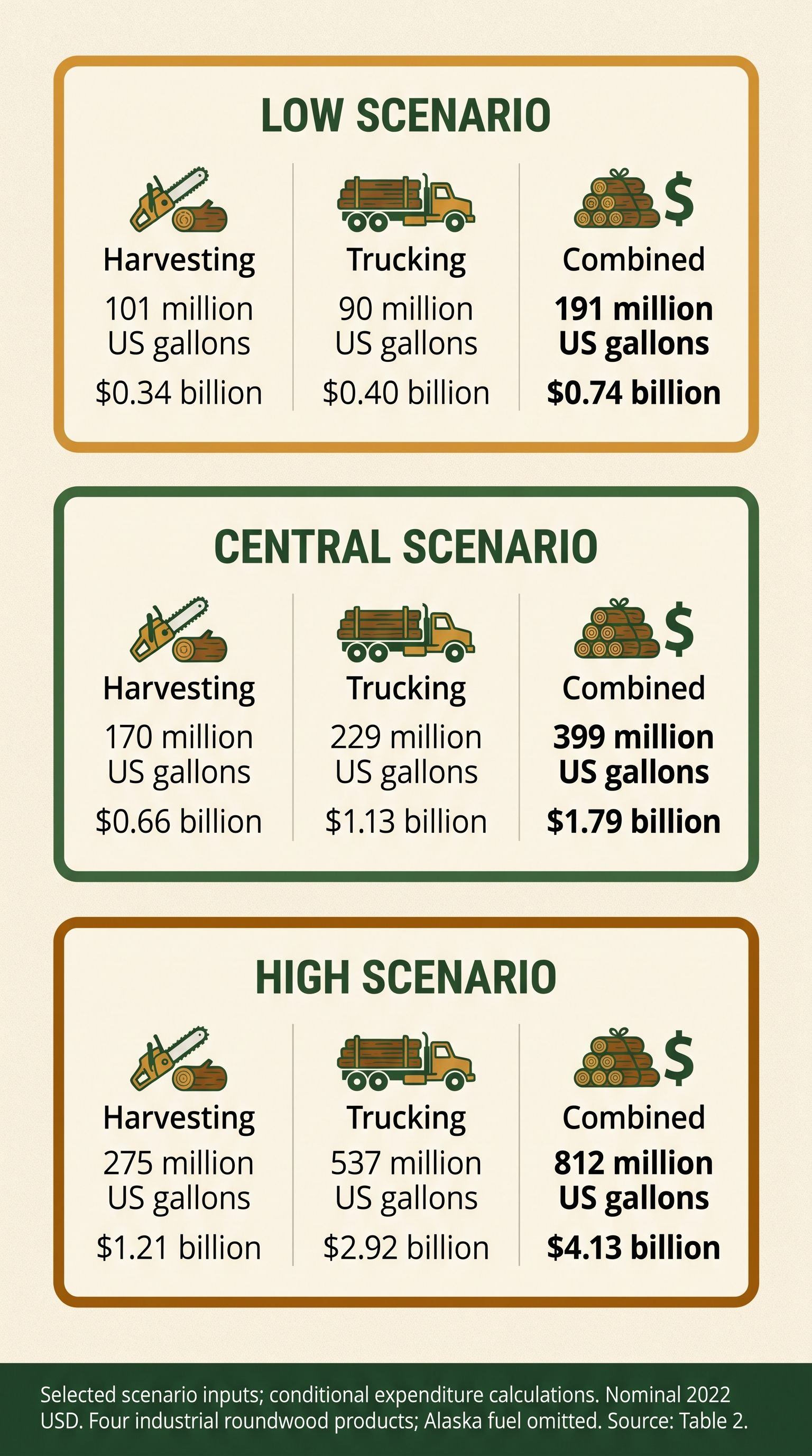
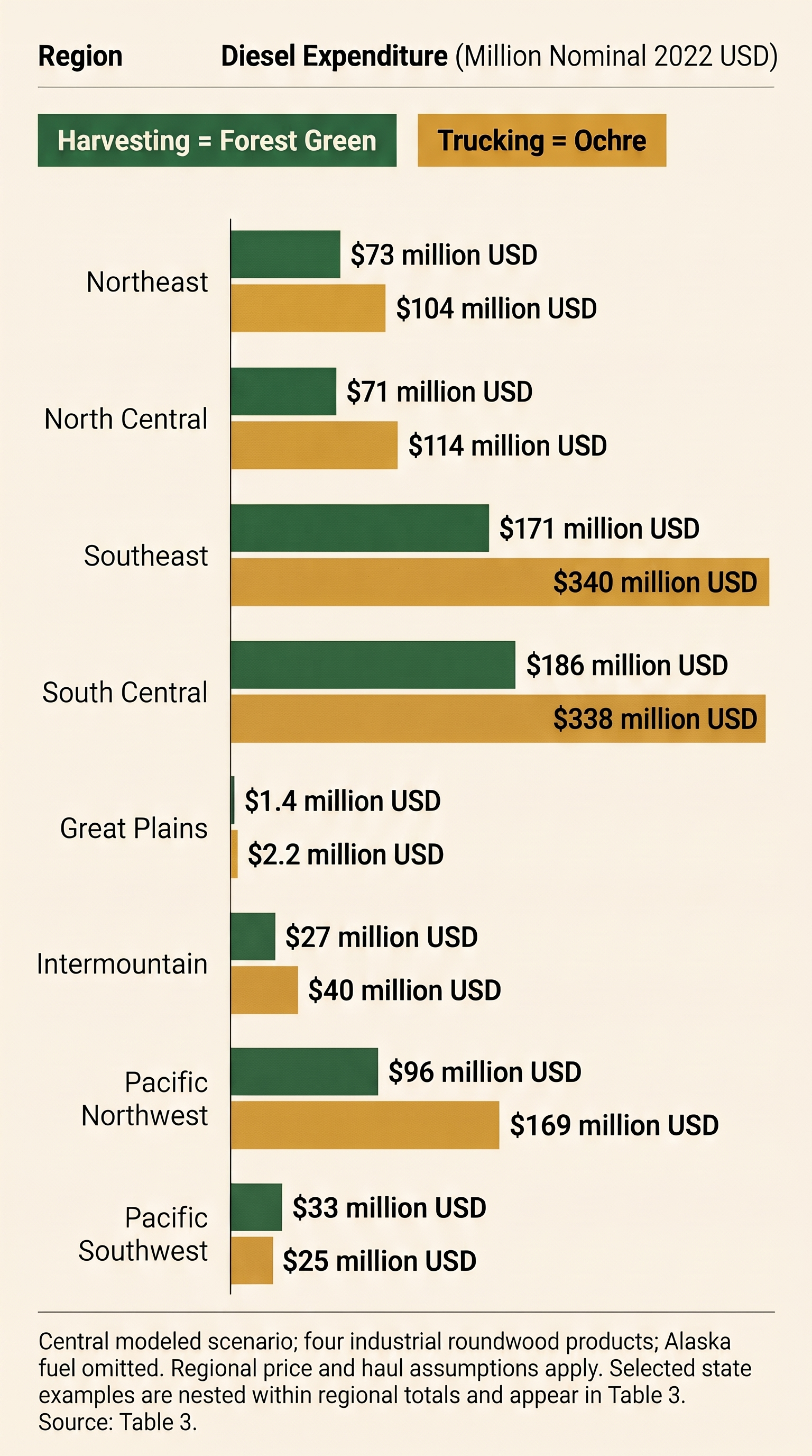
Table 4 reports the low, central and high national scenarios. Table 5 provides the central regional and nested state cases. The national efficiency rates divide total production by each activity’s gallons. Trucking gallons include empty travel.
| Measure | Low | Central | High |
|---|---|---|---|
| Production, million green short tons | 245 | 291 | 337 |
| Harvesting, million U.S. gal | 101 | 170 | 275 |
| Trucking, million U.S. gal | 90 | 229 | 537 |
| Combined, million U.S. gal | 191 | 399 | 812 |
| Harvesting, green short tons per gal | 2.43 | 1.72 | 1.22 |
| Trucking, green short tons per gal | 2.72 | 1.27 | 0.63 |
| Harvesting, $ billion | 0.34 | 0.66 | 1.21 |
| Trucking, $ billion | 0.40 | 1.13 | 2.92 |
| Combined, $ billion | 0.74 | 1.79 | 4.13 |
Nominal 2022 U.S. dollars. The model excludes Alaska fuel and includes Pacific Southwest as a combined source geography. The calculation also excludes independently priced road-building, mill operations, marine freight and other fuels. Figures are rounded independently. Lower cases combine better equipment or truck productivity, lighter implied wood mass and lower input prices. Higher cases combine poorer productivity, longer loaded trips, more empty mileage, lower payloads and higher prices. Simultaneous extremes illustrate exposure. They carry no statistical confidence level. [S05, S06, S08, S10, S11, S12, S13, S14, S15, S16, S17, S18, S19, S20, S21, S22, S23, S24, S40]
| Geography | Green short tons, M | Woods gal, M | Truck gal, M | Woods $, M | Truck $, M |
|---|---|---|---|---|---|
| Northeast | 23.5 | 19.3 | 19.7 | 73 | 104 |
| North Central, including Lake States | 30.0 | 18.0 | 23.2 | 71 | 114 |
| Southeast | 88.3 | 45.0 | 69.1 | 171 | 340 |
| South Central | 93.1 | 47.5 | 72.1 | 186 | 338 |
| Great Plains | 0.5 | 0.4 | 0.4 | 1.4 | 2.2 |
| Intermountain | 9.6 | 6.7 | 8.0 | 27 | 40 |
| Pacific Northwest | 37.7 | 24.5 | 32.4 | 96 | 169 |
| Pacific Southwest | 8.2 | 8.2 | 4.2 | 33 | 25 |
| Alaska | — | — | — | — | — |
| Alabama, selected products | 27.5 | 14.0 | 21.3 | 54 | 100 |
| Georgia, selected products | 28.0 | 14.3 | 21.7 | 54 | 107 |
Nominal 2022 U.S. dollars. State cases are nested in the national geography and use independent TPO product shares and an editable green-density blend. The state estimates and South pulpwood check show the effect of differing product and mass assumptions. The Great Plains and Intermountain results transfer several operating inputs and have especially weak calibration. No separate Hawaiian fuel figure is available. [S20, S21, S22, S23, S24, S33, S34, S35, S36, S37] Figure 8 presents the regional central expenditure comparison.
Sensitivity and operating expenses
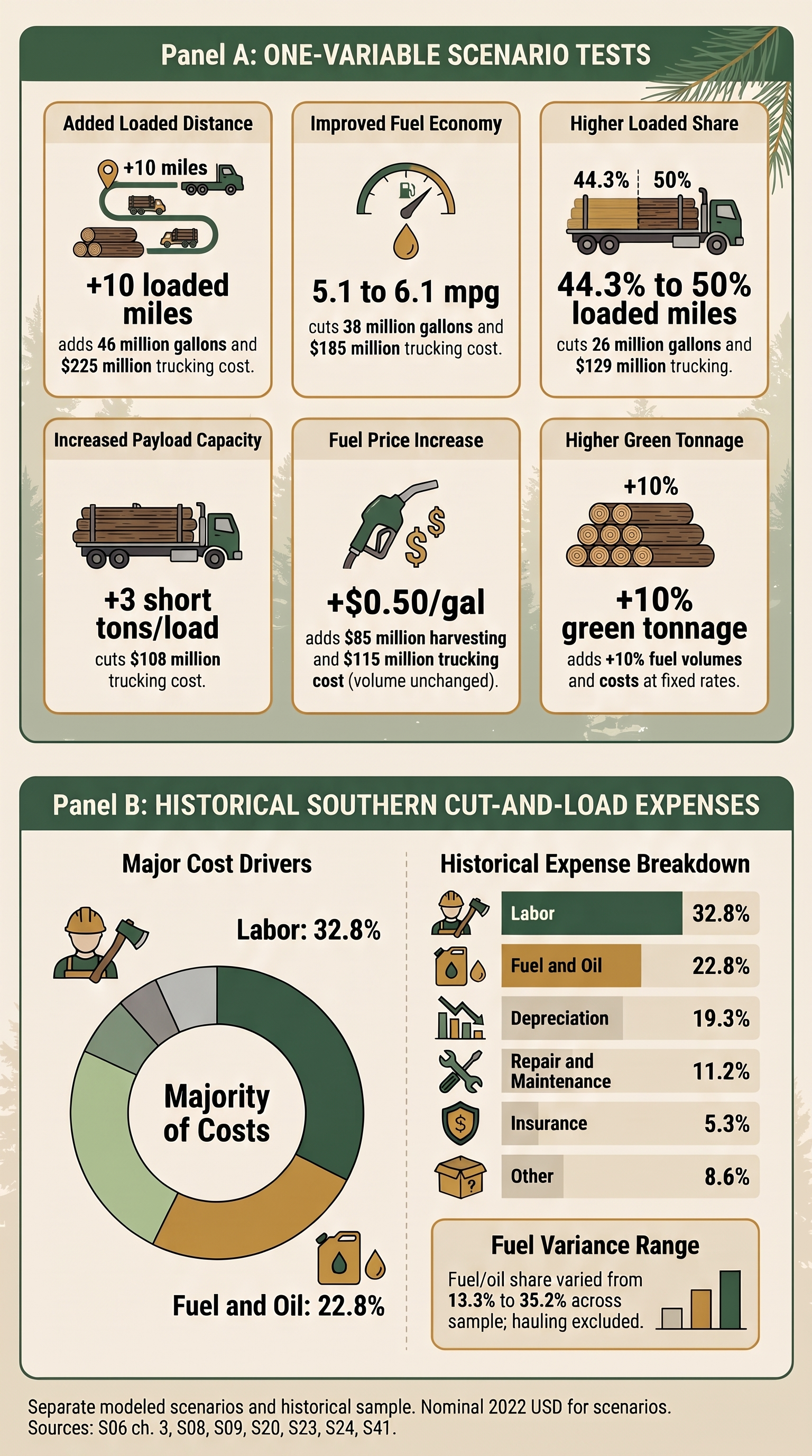
Holding everything else constant, adding 10 miles to the loaded haul in each modeled area adds about 46 million trucking gallons and $225 million. Raising fleet fuel economy from 5.1 to 6.1 mpg reduces trucking by about 38 million gallons and $185 million. Moving from 44.3% to 50% loaded miles lowers trucking by about 26 million gallons and $129 million, with the same distance, payload and fuel economy. A $0.50 increase per gallon adds approximately $85 million for woods diesel and $115 million for trucking. Changing converted green tonnage by 10% changes both annual stages by 10% where intensity and haul are held fixed. These calculations isolate each driver. Real routes, equipment and mills often cause several to move together. [S06, S08, S09, S20, S23, S24] The workbook’s payload test indicates that three additional short tons per load reduce modeled annual cost by about $108 million, with other inputs held fixed. Figure 6 brings these sensitivities together with the historical operating-expense examples that follow.
Baker and colleagues’ historical southern cut-and-load sample allocated 32.8% of costs to labor, 22.8% to fuel and oil, 19.3% to depreciation, 11.2% to repair and maintenance, and 5.3% to insurance. Hauling was excluded from those shares. Fuel and oil ranged from 13.3% to 35.2% across the study firms. These observations document cost structure and variation among the surveyed companies before more recent changes in fuel and equipment costs. [S06, S03, S41]
For trucking, fuel sits alongside wages and benefits, repairs, maintenance, tires, equipment ownership and insurance. Representative company fuel shares require consistent denominators. In Washington, Mason and colleagues’ single-truck owner-operator model estimated nonwage cost of $1.14/mi at the 2006 fuel price and $1.58/mi at the June 2008 price. At 5.1 mpg, fuel alone was about $0.54 and $0.96/mi, respectively. The inferred fuel share of nonwage cost therefore rose from roughly 47% to 61%, before including wages. Conrad’s southern trucking simulation used $30.60/hour in wages and benefits in one case and a separate $21.99/hour assumption for truck and trailer ownership, maintenance, insurance and tires. These historical examples describe their particular trucking settings; a current national logging-business cost breakdown would require broader matched data. [S06, S08, S17, S39]
Contractor calculators
The Forest Business School reviewed Steve Bick’s Wood Takes Fuel beta. The tool helps a contractor estimate how a change in fuel price affects unit costs for six wood-product groups. The operator enters weekly loads, units and load sizes, total weekly gallons and a change in dollars per gallon. The served formulas convert output into common ton equivalents, multiply weekly gallons by the change in price and allocate the result by converted tonnage. The beta uses fixed factors for certain board-foot and cord units, including 4.6 tons per thousand board feet for hardwood sawlogs and 2.5 tons per cord for hardwood pulpwood. This means an operation’s output mix, local conversion factors and the operator’s choice of which gallons to enter affect the result. Separate woods and truck entries would be needed to make a stage comparison through this method. [S30]
The beta was built for the Vermont logger peer group. The project is seeking funding for a version that is easier to use, can accommodate more operations and regions, and can be distributed free to anyone who can use it. The current interface identifies the app as an early test version. It measures the cost effect for the user’s inputs. Its scope is the user’s operation and entered fuel and production data. Conrad’s published adjustment method offers a complementary tract-level approach, with explicit separation of in-woods equipment, support vehicles and trucks. [S09, S30]
6. Farm and non-farm timber
Table 6 distinguishes the available farm, forest-output and administrative concepts and the limits of what each can establish.
| Concept | What the source measures | What can be inferred |
|---|---|---|
| Agricultural census farm | An operation meeting the census test of at least $1,000 in agricultural products normally sold or that could have been sold during the census year. It reports land operated and woodland categories. | Woodland in an agricultural operation can be counted under census rules. Acreage alone gives neither harvested tonnage nor the share of fuel used for timber. |
| Forest-product receipts from farms | Gross forest-product receipts in the census farm-related-income schedule. Christmas trees, short-rotation woody crops and maple products have other categories. Farm expenses pool fuels across activities. | Dollar receipts provide partial evidence of commercialization. Stumpage sales, contract activity and delivered wood have different payment and cost structures. Dividing receipts by a general log price cannot recover fuel use. |
| FIA and TPO | FIA plots estimate forest resources and removals. TPO estimates primary product output and movement by origin and other attributes, including broad ownership. | Public/private and corporate/family categories track ownership. They do not identify a tract as part of a farm operation for program purposes. Receipts at mills also differ from harvest at origin. |
| Woodland-owner survey | Forest ownership and management attributes, including some reported harvest activity. | Ownership or a farming occupation cannot establish whether the specific timber tract belongs to an agricultural operation or how its logger purchased fuel. |
| FSA administrative farm and tract | Part 718 defines farm records around separate operations and tract arrangements. The HFR solicitation describes the activity it seeks to document. | The application of that administrative definition, the allowed activities and eligible claimant would require HFR instructions specific to timber if timber is included. |
Sources [S01, S21, S25, S26, S27, S28, S43].
The 2022 agricultural census counted 72.07 million woodland acres in farm operations, including 24.31 million acres pastured and 47.75 million acres not pastured. It also recorded $1.136 billion in forest-product receipts from 46,260 farms. The receipts exclude cultivated Christmas trees, maple products and short-rotation woody crops. These totals describe land and income under census definitions. Neither total assigns timber production, fuel or a claimant to a specific tract. [S25, S26, S43]
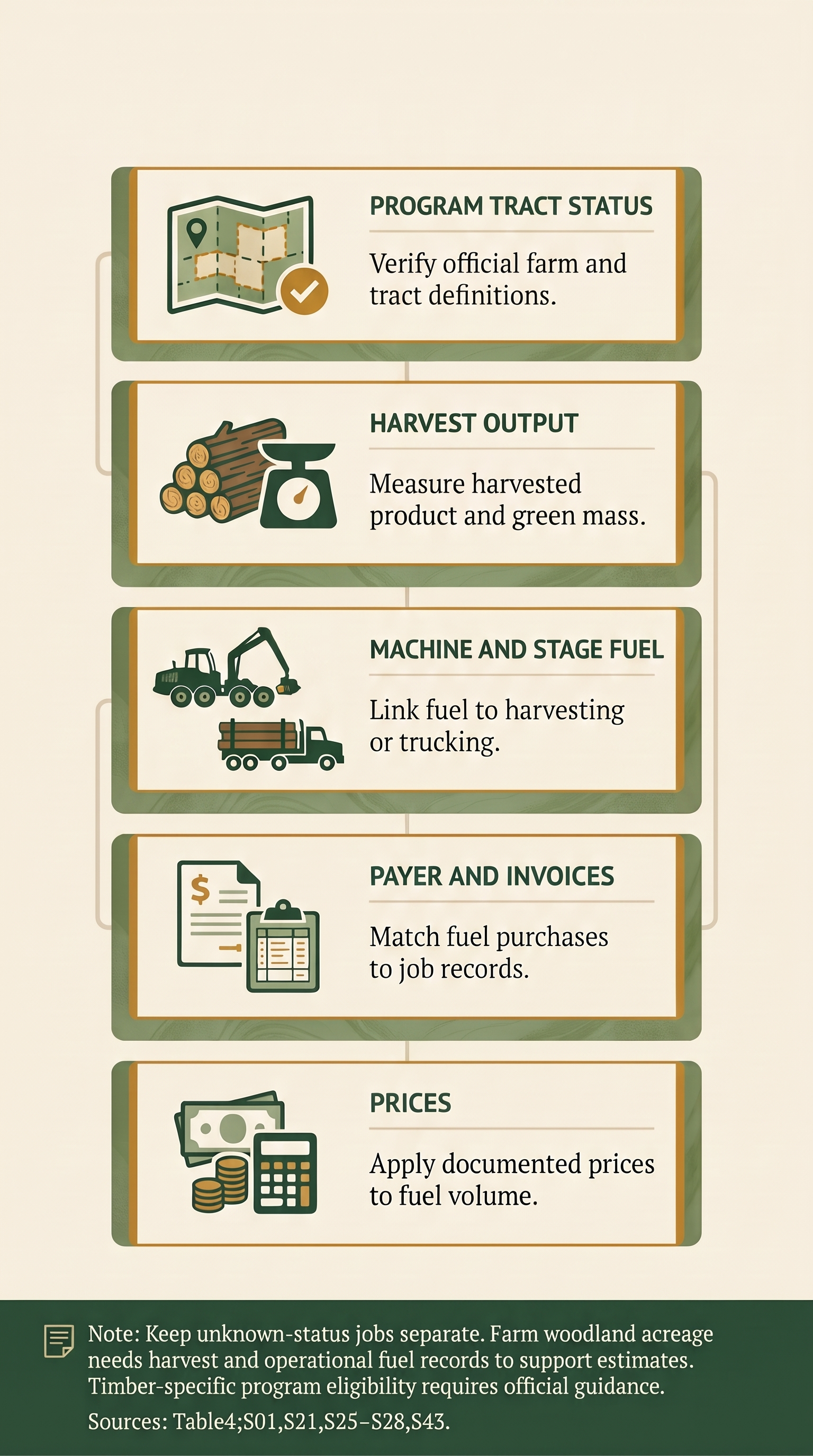
A defensible estimate would classify tracts under the relevant program definition, then estimate harvest tons and fuel intensity by region, system and product within each farm-status category. Match contractor fuel and output to jobs using mill or landing records, and apply buyer invoice prices or a documented common series. Keep unknown-status jobs separate and report their volume and share of missing records. Crews can work in both categories during a week, so tagged activity or gallons provide a stronger allocation basis than acreage or uniform fuel intensity. Existing acreage, receipts, output and separate fuel records lack this direct farm-status linkage. Figure 9 identifies the records to match.
7. Policy briefings
Questions for policymakers and highest-priority missing information
A decision-ready request would specify the eligible commodity and claimant, the tract definition and documentation, and the point where covered production ends. It would establish whether purchases or consumption are counted, what time period applies, and how owner-operated work, contract harvesting and shared equipment are handled. Logs moved to a landing and logs hauled to market should be identified separately in the data, whatever boundary USDA ultimately adopts. Contractor receipts, taxable and dyed diesel invoices, fuel surcharges and a landowner’s stumpage receipt answer different parts of the question. [S01, S21, S25, S26, S27, S28, S29]
Original correspondence and timber-specific instructions. Obtain the original Chappell email PDF and complete wording of the request to document what was requested, by whom and under which farm definition.
A matched 2025–26 contractor and tract sample. Collect green tons, fuel by machine and stage, invoices, land designation, harvest treatment, operators and payer. Draw groups by region, system and contractor size. Include small operators and firms that subcontract haul.
Reconciled product and green-weight data. Obtain origin-based TPO product tables and contemporary payload or weigh-ticket factors, particularly for southern roundwood pulpwood. Document bark, moisture and product equivalence.
Recent haul and fleet records. Identify actual one-way and empty miles, route and grade, price paid, payload, subcontractor boundary, and truck/rail/water split. Prioritize Alaska, the inland West, the Lake States, California and the Northeast. Retrieve the underlying Northeast association survey and determine what its reported 2.1 gal/ton includes.
Treatment of ancillary and other fuels. Measure road work, equipment moves, support trucks, chipping and aviation where material, and document who pays. Retain each category separately so different program rules can be tested.
8. Conclusions and limitations
Limitations
The scenarios use a common 2022 volume and price basis. Fuel inputs originate in different study years, and several are transferred across regions because matched regional fleet and crew data are scarce. The spread describes the joint effect of scenario choices; statistical sampling uncertainty remains unquantified. Applying one contractor survey or one timber type nationwide would suppress actual differences in equipment, utilization, terrain, log density, product mix and first-haul mode. Lower and higher expenditures can coexist within the same region. Figure 7 shows the expenditure range in Table 4 and the separate harvesting and trucking components.
The modeled dollars value calculated gallons at price proxies. Actual business payments, landowner reimbursements and the distribution of the cost burden require invoice and contract evidence. Production reporting is strongest for industrial roundwood groups. Comparable fuel and production records are especially limited for the Plains, Alaska and Hawaii. Separating support and mobile equipment, landing chipping and intermodal freight would change which stages and gallons enter each estimate.
The Northeast archival cases demonstrate why local fuel evidence should retain product mix, support work, fuel type and production conversions. Their seven jobs and two periods describe the participating businesses; pooling would disproportionately weight the larger Maine case. Contractor-reported totals may reflect purchase and inventory timing. Program-eligibility analysis would also require farm-status classifications matched to these records. The U.S. scenario coefficients and annual expenditure totals remain unchanged, with the archive cases reported separately. [S53, S54, S55, S56]
The 0.51-gallon rate provides a documented historical reference for in-woods timber harvesting in parts of Alabama and Florida. The best southern trucking evidence gives a comparable reference near 0.8 gal/ton under its haul and payload conditions. Use both figures with the production systems, geography, dates and operating boundaries that produced them. Local evidence elsewhere shows how much those conditions can change over a working season, within a state or from one tract to the next.
The national scenarios show the scale of industry diesel use and the importance of trucking in commercial costs. For HFR, the evidence priorities are narrower. The public request concerns production fuel on farms, and the currently available data cannot tie a national farm or non-farm volume to fuel used by the party incurring the expense. Matched tract, contractor and fuel records could close that gap and allow separate estimates by stage.
THE EVIDENCE EXPLORER
Regional evidence explorer
Select a region to compare study results, sample coverage and the work included in each estimate.
All gallon conversions use U.S. gallons. Original study units are retained where a mass conversion is not defensible. Tons mean 2,000-lb short tons; “green” means as-received wood including moisture. A volume-based result cannot become gallons per ton without a defensible mass conversion.
THE FUEL WORKBENCH
Fuel and cost calculators
Enter fuel records, production, payload and route information to calculate fuel intensity and cost. The examples show how each assumption affects the result.
Distance, payload and empty travel
Empty travel and payload can change fuel per ton even when the truck’s fuel economy stays the same.
YOUR ILLUSTRATIVE HAUL
0.81U.S. gallons / green short ton1.23tons / gallon
$3.25fuel / delivered ton
Loaded miles 50 · Other miles 64
Show the calculation & limits
Gallons/ton = loaded distance ÷ loaded share ÷ mpg ÷ payload. Fuel cost/ton = gallons/ton × price.
MPG represents average fuel economy across all travel. Loaded share measures the fraction of total miles traveled with a load. This calculation covers travel fuel; idling, loading and other operating expenses require separate records. Rounded defaults draw on historical Southern trucking research [S06, S08].
Harvesting fuel and annual production
Test an operating assumption or enter a measured rate from your own fuel and production records.
YOUR ILLUSTRATIVE WOODS OPERATION
25,500U.S. gallons / year$102,000annual fuel spending
1.96tons / gallon
Show the calculation & limits
Annual gallons = rate × production. Annual fuel spending = gallons × price. The default 0.51 gal/ton comes from six historical Alabama/Florida crews [S05]. Its applicability depends on the harvesting system and conditions. Trucking, additional support fuel and other operating costs require separate estimates.
Metric evidence. Comparable units.
Conversion requires the reported fuel intensity and a matching wood density. Record the source of the density and retain the original study units.
YOUR CONDITIONAL DIESEL CONVERSION
1.001U.S. gallons of diesel / green short ton0.999tons / gallon
0.975gallons / m³
Show the calculation & limits
Gallons/short ton = (L/m³ ÷ 3.785411784) × (907.18474 ÷ kg/m³).
The default uses 3.69 L of diesel per m³ and the New Brunswick study’s 883 kg/m³ green-log transport density as a proxy [S49]. The result applies to that company case under the stated density assumption. Dry mass, green mass, solid wood volume and loose chip volume each require their own conversion basis.
RESEARCH LIBRARY
A briefing for your region
Explore the source collection in NotebookLM and ask for a custom report focused on your region, harvesting systems and policy questions.
Open the research notebook →Compiled using resources supplied by The Forest Business School. Verify generated reports against original sources and retain their units, dates and operating boundaries.
“What can the evidence support about harvesting fuel in the Lake States, and where are local records still needed?”
The notebook includes source material at different levels of completeness, including some abstracts and index pages. Its source notes record coverage and access limits. Correspondence and restricted contractor research are excluded.
TRACE THE CLAIM
References and source notes
Open the original source. Check its date, geography, sample and operating boundary before reusing a number.
Open the complete bibliography · All 56 reference entries on a separate, printable page.
The source notes distinguish published studies, abstracts and attributed unpublished summaries. Contractor identities and underlying business records remain private.
Complete bibliography
S01 USDA Farm Service Agency, Harvest Fuel Relief (2026). Original reference · check scope and date
S02 USDA announcement, October 19 (2026). Original reference · check scope and date
S03 New Jersey Department of Agriculture fuel-data request (2026). Original reference · check scope and date
S04 WXPR, reporting on logging relief (2026). Original reference · check scope and date
S05 Jonathan Kenney, Auburn University MS thesis (2015). Original reference · check scope and date
S06 Shawn A. Baker, University of Georgia doctoral dissertation, ch. 4 (2015). Original reference · check scope and date
S07 Kenney and colleagues, Factors that Affect Fuel Consumption in Logging Systems (2014). Original reference · check scope and date
S08 Joseph L. Conrad IV, Evaluating Profitability of Individual Timber Deliveries (2021). Original reference · check scope and date
S09 Joseph L. Conrad IV, Fuel Cost Adjustments (2022). Original reference · check scope and date
S10 Richard Root and Jeff Benjamin, ECANUSA proceedings (2008). Original reference · check scope and date
S11 Zhao and coauthors, Eastern hardwood forest resources LCA (2024). Original reference · check scope and date
S12 Blinn and colleagues, Status of the Minnesota Logging Sector in 2021 (2023). Original reference · check scope and date
S13 Bowe and colleagues. The Logging Sector in Minnesota and Wisconsin: Status, Issues, and Challenges in 2021 (2025). Original reference · check scope and date
S14 Professional Logging Contractors of the Northeast, Logger’s Voice (2026). Original reference · check scope and date
S15 Han and coauthors, Northern California redwood life cycle (2015). Original reference · check scope and date
S16 CORRIM Module A, Forest Resources (2004). Original reference · check scope and date
S17 Mason and colleagues, Washington Log Trucking Industry (2008). Original reference · check scope and date
S18 CORRIM, Inland Northwest Softwood Lumber (2024). Original reference · check scope and date
S19 USDA Forest Service, Logging Utilization in Alaska (2022). Original reference · check scope and date
S20 Oswalt and colleagues, Forest Resources of the United States 2022 (2026). Original reference · check scope and date
S21 USDA Forest Service, NRUM / TPO data and methods (2026). Original reference · check scope and date
S22 USDA Forest Service, Southern Pulpwood Production 2022 (2024). Original reference · check scope and date
S23 U.S. EIA, Retail Prices for Diesel On-Highway (2026). Original reference · check scope and date
S24 U.S. EIA, State Energy Data System distillate prices (2026). Original reference · check scope and date
S25 USDA NASS, 2022 Census of Agriculture (2024). Original reference · check scope and date
S26 NASS, 2022 Census of Agriculture reporting guide (2022). Original reference · check scope and date
S27 7 CFR 718.2, definitions (2026). Original reference · check scope and date
S28 National Woodland Owner Survey, Family Forest Research Center (2026). Original reference · check scope and date
S29 IRS, 2026 dyed diesel relief (2026). Original reference · check scope and date
S30 Steve Bick / Northeast Forests LLC, Wood Takes Fuel beta (2026). Open beta Original reference · check scope and date
S31 Abubakar Tahiru, Auburn University MS thesis (2025). Abstract / record only
S32 Smidt and colleagues, Trucks-to-trucks (2025). Original reference · check scope and date
S33 University of Montana BBER, Black Hills processing capacity (2024). Original reference · check scope and date
S34 Maher and colleagues, Northwest Forest Industries data series (2026). Original reference · check scope and date
S35 Chappell email attachment described in supplied correspondence Private correspondence; bibliographic context only.
S36 USDA FS 2022 Alabama TPO fact sheet (2024). Original reference · check scope and date
S37 USDA FS 2022 Georgia TPO fact sheet (2024). Original reference · check scope and date
S38 Maine Forest Service annual reports and processor series (2026). Original reference · check scope and date
S39 Wallace Economic Advisers and PLC Northeast economic contribution (2026). Original reference · check scope and date
S40 US Forest Products Laboratory, Wood Handbook (2021). Original reference · check scope and date
S41 Baker, Mei, Harris and Greene, Index for Logging Cost Changes (2014). Original reference · check scope and date
S42 Hawaii DLNR Division of Forestry and Wildlife, Local Wood Products (2026). Original reference · check scope and date
S43 National Agricultural Statistics Service, Census Tables 7 and 8 (2024). Original reference · check scope and date
S44 U.S. Census Bureau, North American Industry Classification System (2022). Original reference · check scope and date
S45 Bick, Steven. 2015. Energy Returned on Energy Invested for Woody Biomass Heating Fuels in New York State. Unpublished paper, Northeast Forests, LLC, October 28. Author-supplied study commissioned by NYSERDA; published here as an attributed summary. Underlying document remains unpublished.
S46 Athena Sustainable Materials Institute. 2009. A Cradle-to-Gate LCA of Canadian Softwood Lumber. Sections 4.1–4.1.1 and Table 4, pp. 23–25. Original reference · check scope and date
S47 Athena Sustainable Materials Institute. 2018. A Cradle-to-Gate LCA of Eastern Canadian Surfaced Dry Softwood Lumber. Section 4.2 and Table 4. Original reference · check scope and date
S48 Athena Sustainable Materials Institute. 2018. A Cradle-to-Gate LCA of Canadian Surfaced Dry Softwood Lumber. Section 4.2 and Table 4. Original reference · check scope and date
S49 Zahabi, Gong, Gu and Blackadar. 2025. The Cradle-to-Gate Life Cycle Assessment on Hardwood Lumber Production in New Brunswick, Canada. Buildings 15(3), 499. Sections 2.2–2.2.2 and Table 1. Original reference · check scope and date
S50 Labelle, Yadegari and LeBel. 2025. Evaluating fuel consumption and productivity of hybrid harvesters operating in eastern Canada. COFE conference abstract. Abstract / record only
S51 Iyer and colleagues. 2025. The Use of Hybrid Trucks in Forest Transports. HVTT18 conference paper, pp. 2–5. Original reference · check scope and date
S52 Environment and Climate Change Canada. 2026. Fuel LCA Model Methodology. September edition, section 3.5.5. Original reference · check scope and date
S53 Quinn, Ha, Volk, Brown, Bick, Malmsheimer and Fortier (2020). Life cycle assessment of forest biomass energy feedstock in the Northeast United States. GCB Bioenergy 12:728–741. Full text and public supplement examined; related research family
S54 Ha and colleagues (2022). Economic feasibility of forest biomass feedstock supply chains: clean and dirty chips for bioenergy applications. Biofuels, Bioproducts and Biorefining 16:389–402. Metadata and abstract examined; full methods not verified
S55 Ha and colleagues (2024). A Stochastic Techno-Economic Analysis of Forest Biomass Feedstock Supply Chains: Clean and Dirty Chips for Bioenergy Applications. BioEnergy Research 17:1739–1754. Metadata and abstract examined; full methods not verified
S56 Bick ESF-DOE contractor archive (2026 reanalysis). Selected anonymous New York 2017–2020 and Maine 2017 records. Anonymous aggregate case summary only; underlying business records private. Not a representative sample.
FROM RESEARCH TO PRACTICE
The Wood Takes Fuel app
The Wood Takes Fuel (WTF) beta app supports practical wood-fuel questions. Further development will expand its coverage and improve its usefulness for forest businesses.
Try the WTF beta →